Finite differences with simultaneous perturbation

Need for computing gradients

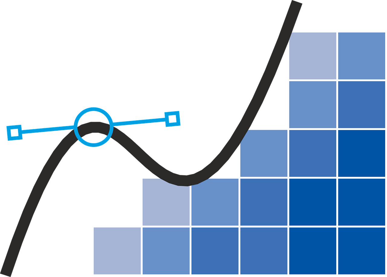
Gradient descent is one of the most popular optimization algorithms used to optimize many machine learning models. The core idea behind the gradient descent algorithm is to compute the gradient of the loss or an objective function with respect to its parameters and iteratively update these parameters towards the direction that will minimize the loss. Throughout my journey as a research student, I have often encountered objective functions with high dimensional parameter space where computing an analytic expression for the derivative becomes difficult. Ofcourse, with the advent of deep neural networks as an effective non-linear function approximator and the availability of some excellent frameworks to implement them, we naturally do not have to worry about computing the gradient of the loss function. This is automatically done using automatic differentiation packages which computes the gradient using chain rule.

Computing gradient with finite differences

Finite differences is one of the oldest method used to solve differential equations. These methods are well understood where the central idea is to evaluate the objective function for two different parameter values and dividing them by their difference.

Consider the objective function defined as \(h(\theta)\), where \(\theta\) is the parameter of the function. Let \(\alpha = \theta+\epsilon\). Therefore the derivative of \(h\) at point \(\theta\) is given by the limit

[\begin{aligned}h’(\theta)= \lim_{\epsilon\to 0}\dfrac{h(\alpha)-h(\theta)}{\epsilon}\end{aligned}]

I had some experiences of using finite difference methods for performance gradient estimation with Partially Observable Markov Decision Processes (POMDPs). Since I was using a stochastic finite state controller for POMDPs it was not straight forward for me to compute the performance gradient analytically. Therefore I used two finite difference algorithms.

Simultaneous Perturbation Stochastic Approximation (SPSA) [1].
Smooth Function Approximation (SFA)[2].

These two algorithms fall in the family of simultaneous perturbation algorithm where the gradient estimate \(\widehat\nabla h\) takes the form

[\begin{aligned}\widehat\nabla h = \dfrac{\delta \Bigl(h(\omega)-h(\theta)\Bigr)}{k}\end{aligned}]

where \(\omega = \theta + k\delta\) and \(k\) is a small constant. \(\delta\) is a random variable with the same size of \(\theta\). The subtle difference between these two algorithms is the way \(\delta\) is generated. For SFA, \(\delta\) is sampled from a normal distribution,i.e., \(\delta\sim \mathcal N(0,I)\) with \(I\) being identity matrix. For SPSA \(\delta\) is sampled from a Rademacher distribution \(\delta^{(i)}\sim Rademacher(+1,-1)\) (where \(\delta^{(i)}\) has \(0.5\) probability of being \(+1\) and \(-1\)) respectively.

Practical experience and limitations

My practical experience in using both these algorithms is quite similar. Both these algorithms are fairly easy and straightforward to implement. One of the limitations of using both these algorithms or any finite difference algorithms in general is that you need to evaluate the objective function twice with different parameters. This can get expensive if the function evaluation is itself expensive. The main takeaway from these family of algorithms is that they only provide an approximate estimate of the gradient. Thus, they might not work well if an algorithm requires an exact gradient computation. Nevertheless they provide a neat way of gradient estimation and are widely used for large-scale population models, simulation optimization and atmospheric modelling.

References

Spall, J. C. (1992). Multivariate stochastic approximation using a simultaneous perturbation gradient approximation. IEEE transactions on automatic control, 37(3), 332-341.
Katkovnik, V. Y., & KULCHITS. OY. (1972). Convergence of a class of random search algorithms. Automation and Remote Control, 33(8), 1321-1326.